A simple physics simulation
Abstract
This first tutorial is intended to familiarize you with the simulator if you had not used it before. One goal is to show the basic spatial and temporal navigation functions as well as information displays. For this purpose, we want to load an existing simulation file from the examples provided. For the sake of simplicity, we will choose an example here where the cell clusters do not perform any additional actions. In general, it is possible to equip them with functions that allow programmable interaction with the environment.
What you will see
1. Open an existing simulation
We open a prepared simulation by clicking on Simulation in the menu and then on Open. We go to the directory ./examples/simulations and open obstacles.sim. Generally, every simulation consists of 4 files. In this case we have the following:
- obstacles.sim - This is the main file, visible only in the selection. It contains everything that is inside the simulated world.
- obstacles.settings.json - The general settings (world size and CUDA settings) are stored here. They are encoded in JSON (JavaScript Object Notation) and can thus be edited outside with any editor.
- obstacles.parameters.json - This JSON file contains the simulation parameters. These include, among others, physical values indicating damage, fusion or energy radiation of bodies.
- obstacles.symbols.json - Here you find a list of symbols and their defining values. The symbols are auxiliary constructs and are used for writing small programs in a certain assembler-like language. They can be constants or variables. The programs can be linked to a cell and are executed when triggered.
2. Spatial navigation
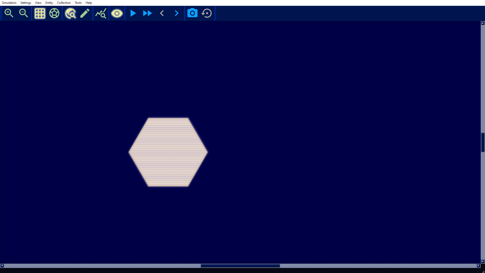
After loading the simulation the view is centered, the zoom level is set to 4x and the simulation is paused. On the bottom you see information about the file (world size, number of different types of entities, etc.). However, in this initial setting, you will not see as much in this example, probably that:
By default, the navigation mode is enabled. This meant that we can navigate with the mouse as follows:
- If we press and hold the left mouse button, we zoom in the direction of the mouse cursor.
- If we press and hold the right mouse button, we zoom out.
- If we press and hold the middle mouse button, we can scroll by moving the mouse.
Regardless of this, we can click on the magnifying glass icon and scroll using the scroll bar. For a better view, we zoom out to zoom level 1x by clicking on the appropriate magnifying glass icon and then scrolling up.
The simulator provides three different types of rending modes which are automatically changed after zooming:
- item mode: With zoom level 16x or larger the clusters and particles are visualized with all details. Tokens, bonds between cells and cell functions (shown when cell info is enabled) are displayed. In addition, all available editing options are unlocked: Selections can be made and physical values (velocities, angular velocities, bonds, energies....) can be changed via input fields or with the mouse cursor. Some of these functions are displayed on icons in a second toolbar that overlays the view.
- vector mode: Between zoom level 4x and 8x the elements are rendered in a vector graphic style. More precisely, cells, particles and bonds are rendered. Tokens are also visible as glowing circles.
- pixel mode: At zoom level 2x or lower, the objects are rendered as points.
3. Temporal navigation
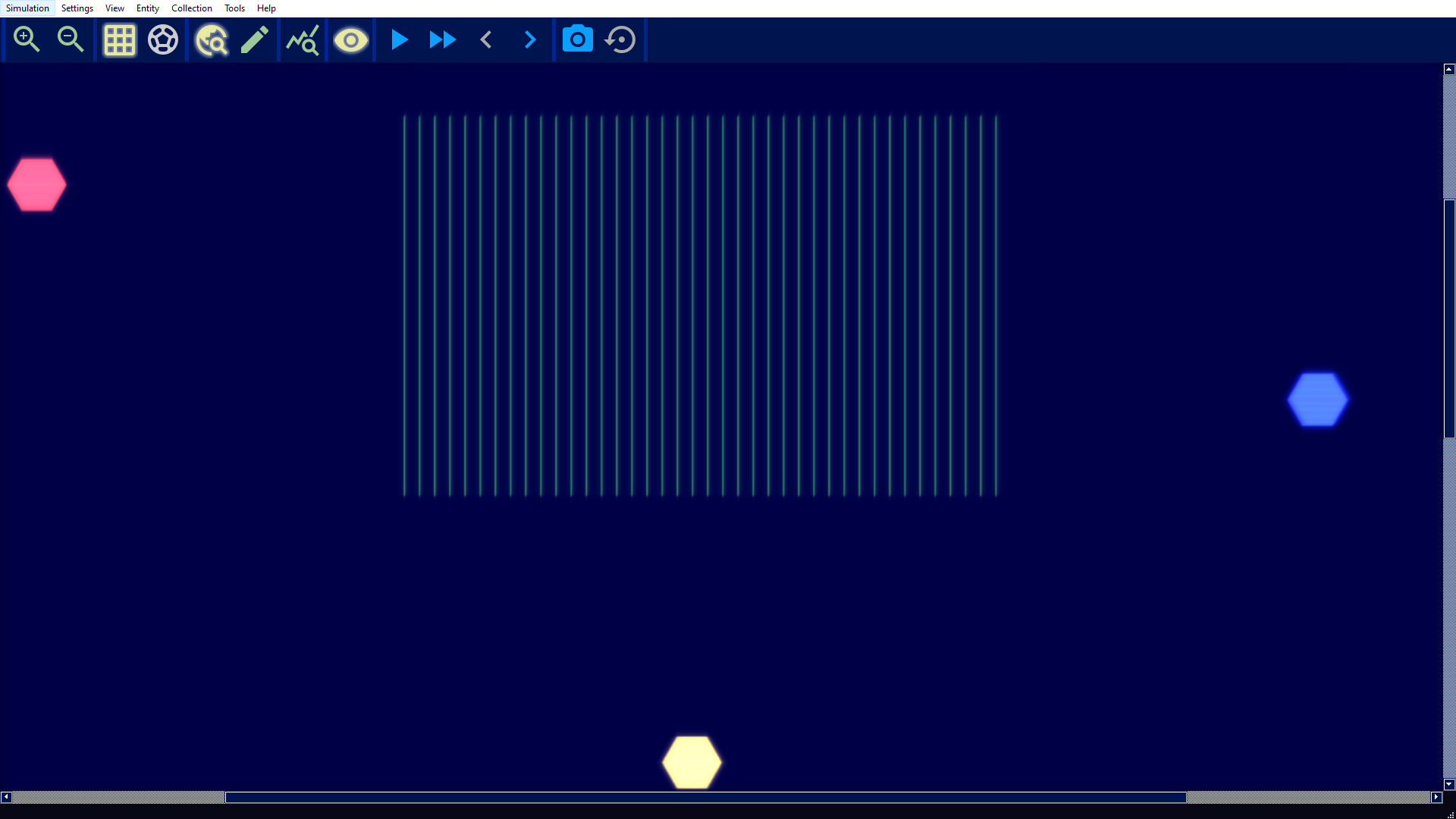
We are now able to start the simulation by clicking on the play icon. After that, you should probably see something similar to the video above. In the info bar at the bottom you can see the number of time steps that will be calculated. Clicking this toolbar button again (which is now a pause icon) will pause the simulation. alien offers several functions to navigate through time:
- move a single time step forward: This function can be reached via the > button.
- move a single time step backward: This function can be reached via the < button. This only works if a single time step has been calculated beforehand.
- make snapshot: The entire world is stored in the memory. This function can be accessed via the camera button. Note that only one snapshot can be taken. Clicking the camera again will delete the previous snapshot.
- restore snapshot: When a snapshot is created, you can click the Restore button. Then the snapshot will be loaded. This also works in a running simulation (... and is fun! Please try it.). A snapshot can be reused, or in other words, it will not be deleted after restoring.
And for the sake of completeness:
- accelerate: It is possible to focus most computational resources on cell clusters that have tokens. In some simulations (but not in this one), these may be the clusters of greatest interest. This feature will be covered in more detail in another tutorial.
An additional acceleration of the calculation can also be achieved by switching off the rendering. To do this, click the eye button ("disable display link").
Created with the Personal Edition of HelpNDoc: Full-featured EPub generator